Profiling Parallel Applications
Overview
Teaching: 30 min
Exercises: 30 minQuestions
It works, but what is taking time?
Objectives
Use a profiler to find bottlenecks and hotspots and diagnose problems.
| Display Language | ||
|---|---|---|
Profiling
Profilers help you find out where the program is spending its time and pinpoint places where optimising it makes sense. In this lesson we will use Scalasca, but many other profilers exist. Scalasca is specifically an MPI profiler; it will give you information on communication efficiency and bottlenecks.
Scalasca is an open source application developed by three German research centers. For more information check the project website.
It is used together with the Score-P utility, the Cube library
and the Cube viewer.
Since it is open source, you can install it in your home directory on any HPC cluster
that does not already have it.
The process is as described in setup, but you need to add
--prefix=$HOME/scalasca/ to the ./configure command to install in
your home folder.
Summary profile
It is advisable to create a short version of you program, limiting the runtime to a few minutes. You may be able to reduce the problem size or required precision, as long as this does not change the algorithm itself. We will use the Poisson solver from the previous lesson as an example. The example program used here (and at the end of the previous section) is here here.
Later we will see how we can limit the scope of the profiler, but first
we need to run a summary of the whole program.
Start by recompiling the application, replacing mpicc with the version
provided by the Score-P utility.
Assuming the final version is saved into poisson.c it is compiled with:
scorep mpicc -o poisson poisson.c
Assuming the final version is saved into poisson.F08 it is compiled with:
scorep mpifort -o poisson poisson.F08
This will produce an instrumented binary. When you execute it, it will track function calls and the time spent in each function.
Next, run the new executable using Scalasca to analyse the data gathered:
scalasca -analyze mpirun -n 2 poisson
Finally, you can examine the results in the GUI:
scalasca -examine scorep_poisson_2_sum
This will open cubeGUI.
If you are running the GUI on a cluster over a normal internet connection,
it may be slow and unresponsive.
It’s usually faster to copy the data folder (here scorep_poisson_2_sum)
to your computer and run the GUI there.
Profile Your Poisson Code
Compile, run and analyse your MPI version of the poisson code. How closely does it match the performance below? What are the main differences?
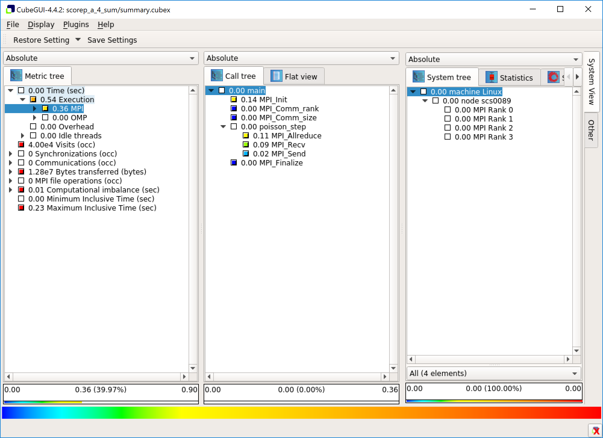
The GUI has three panels: a metric view, a function view and a system view. In the metric view you can pick a metric to be displayed. You can dig into the details of some of the metrics in a tree view. The second panels shows functions either as a call tree, displaying which functions have called what, or as a flat view. It also displays the metric you have chosen on a function level. The system view displays data on the chosen function on a deeper level.
Right clicking on the view and choosing “Info” replaces the system view with an info view. This gives information on the chosen metric.
If you are running on a cluster you may wish to use the command line instead.
To supress the GUI, use the -s parameter:
scalasca -examine -s scorep_poisson_2_sum
cat scorep_poisson_2_sum/scorep.score
The command line version will produce output that looks something like this:
Estimated aggregate size of event trace:                   501kB
Estimated requirements for largest trace buffer (max_buf): 251kB
Estimated memory requirements (SCOREP_TOTAL_MEMORY):       4097kB
(hint: When tracing set SCOREP_TOTAL_MEMORY=4097kB to avoid intermediate flushes
 or reduce requirements using USR regions filters.)

flt     type max_buf[B] visits time[s] time[%] time/visit[us]  region
         ALL    256,161 12,012    4.03   100.0         335.60  ALL
         MPI    232,096 10,008    0.52    12.9          52.03  MPI
         COM     24,024  2,002    3.51    87.1        1753.48  COM
      SCOREP         41      2    0.00     0.0          39.56  SCOREP

         MPI     66,000  2,000    0.30     7.5         151.18  MPI_Allreduce
         MPI     59,000  2,000    0.01     0.3           5.86  MPI_Recv
         MPI     59,000  2,000    0.01     0.1           2.97  MPI_Send
         MPI     24,024  2,002    0.00     0.0           0.11  MPI_Comm_size
         MPI     24,024  2,002    0.00     0.0           0.14  MPI_Comm_rank
         COM     24,000  2,000    3.51    87.0        1753.84  poisson_step
      SCOREP         41      2    0.00     0.0          39.56  poisson
         MPI         24      2    0.00     0.0          42.81  MPI_Finalize
         COM         24      2    0.00     0.1        1392.03  main
         MPI         24      2    0.20     5.0      100037.07  MPI_Init
Either way we find that in our case, the program is waiting for MPI
communication for 13% of the total runtime.
This is not great for only two cores, so we would like to know if we can do better.
87% of the time is spent in poisson_step.
This is not counting the time spent in functions called by poisson step.
This essentially means that 87% of the time is spent in actual computation.
If you are working on a terminal and prefer not to use the GUI, Cube can print most of the information for you For example the following will print out the time spent in each function:
cube_stat -t 20 -p scorep_poisson_2_sum/profile.cubex
This outputs
cube::Region   NumberOfCalls ExclusiveTime InclusiveTime
poisson_step             200      0.551116      0.727231
MPI_Init                   2      0.221584      0.221584
MPI_Allreduce            200      0.154211      0.154211
MPI_Recv                 200      0.020997      0.020997
poisson                    2      0.003256      0.952162
MPI_Send                 200      0.000827      0.000827
poisson                    2      0.000088      0.952250
MPI_Finalize               2      0.000073      0.000073
MPI_Comm_rank            202      0.000057      0.000057
MPI_Comm_size            202      0.000041      0.000041
The INCL(main) includes function calls inside the main function, while EXCL(main) counts only the time spent in the main function itself.
This tells us clearly that poisson_step is the most important function
to optimise.
You can also print a call tree using:
cube_calltree -m time scorep_poisson_2_sum/summary.cubex
This will print a tree view of function calls with timings:
Reading scorep_poisson_2_sum/profile.cubex... done.
7.91242e-05     poisson
0.00278406        + main
0.200074          |   + MPI_Init
1.02831e-05       |   + MPI_Comm_rank
3.21992e-06       |   + MPI_Comm_size
3.50769           |   + poisson_step
0.000271832       |   |   + MPI_Comm_rank
0.000207859       |   |   + MPI_Comm_size
0.302362          |   |   + MPI_Allreduce
0.0117208         |   |   + MPI_Recv
0.00593548        |   |   + MPI_Send
8.56184e-05       |   + MPI_Finalize
The numbers on the left give the amount of time spent in each function.
Options
Try adding the
-iflag tocube_calltree. What does this do?Solution
The percentages have changed to inclusive ones. They now report the whole time spent in the function, including in sub-function calls.
Note on the Windows Subsystem for Linux
Unfortunately the kernel interface provided by the Windows Subsystem for Linux does not support hardware level profiling. If you are running inside the Subsystem you have significantly less information. In a moment we will see ways of getting more information even in this case, but the best option is to run the profiler on an HPC cluster and examine the results on your personal computer.
Filtering
You can probably see that in a larger program the call tree would be large and hard to manage. The graphical interface makes this a bit easier, but the real solution is filtering.
Filtering can be used to turn off measurements in less important parts of
the code or to restrict measurements to the most interesting parts
of the code.
The filter needs to be saved as a file.
The following will filter out everything except poisson_step, effectively
restricting the measurements to this function:
SCOREP_REGION_NAMES_BEGIN
  EXCLUDE
    *
  INCLUDE
    poisson_step
SCOREP_REGION_NAMES_END
Save this to a file called poisson.filter and run:
scorep-score -f poisson.filter -r scorep_poisson_2_sum/profile.cubex
The output is similar to before, but it now includes a filter column:
Estimated aggregate size of event trace:                   501kB
Estimated requirements for largest trace buffer (max_buf): 251kB
Estimated memory requirements (SCOREP_TOTAL_MEMORY):       4097kB
(hint: When tracing set SCOREP_TOTAL_MEMORY=4097kB to avoid intermediate flushes
 or reduce requirements using USR regions filters.)

flt     type max_buf[B] visits time[s] time[%] time/visit[us]  region
 -       ALL    256,161 12,012    4.03   100.0         335.60  ALL
 -       MPI    232,096 10,008    0.52    12.9          52.03  MPI
 -       COM     24,024  2,002    3.51    87.1        1753.48  COM
 -    SCOREP         41      2    0.00     0.0          39.56  SCOREP

 *       ALL    256,137 12,010    4.03    99.9         335.42  ALL-FLT
 -       MPI    232,096 10,008    0.52    12.9          52.03  MPI-FLT
 *       COM     24,000  2,000    3.51    87.0        1753.84  COM-FLT
 -    SCOREP         41      2    0.00     0.0          39.56  SCOREP-FLT
 +       FLT         24      2    0.00     0.1        1392.03  FLT

 -       MPI     66,000  2,000    0.30     7.5         151.18  MPI_Allreduce
 -       MPI     59,000  2,000    0.01     0.3           5.86  MPI_Recv
 -       MPI     59,000  2,000    0.01     0.1           2.97  MPI_Send
 -       MPI     24,024  2,002    0.00     0.0           0.11  MPI_Comm_size
 -       MPI     24,024  2,002    0.00     0.0           0.14  MPI_Comm_rank
 -       COM     24,000  2,000    3.51    87.0        1753.84  poisson_step
 -    SCOREP         41      2    0.00     0.0          39.56  poisson
 -       MPI         24      2    0.00     0.0          42.81  MPI_Finalize
 +       COM         24      2    0.00     0.1        1392.03  main
 -       MPI         24      2    0.20     5.0      100037.07  MPI_Init
The + and - sign denote what is filtered out and what is not.
The * character denotes a region that is partially filtered.
In this case, only the main function is filtered out. Unfortunately we cannot
remove the MPI_Init function. Normally we would run for longer and it would
not matter.
Once you are happy with the filter, it can then be passed to Score-P with the
SCOREP_FILTERING_FILE environment variable:
export SCOREP_FILTERING_FILE=poisson.filter
scorep mpicc -o poisson poisson.c
export SCOREP_FILTERING_FILE=poisson.filter
scorep mpifort -o poisson poisson.F08
Score-P will only instrument and measure the parts of the program not filtered out. This make profiling faster and the results easier to analyse.
Trace Analysis
Let’s now run the application with the full trace using the -t flag:
scalasca -analyze -t mpirun -n 2 poisson
And examine the results written to the scorep_poisson_2_trace directory:
scalasca -examine scorep_poisson_2_trace
There are some new measurements on the left column.
Notably you will find a a measure of MPI_Wait states, how long the ranks spend
waiting for data.
In addition, you will see the number of MPI communications, and the time spent synchronising
ranks.
User defined regions
By default Score-P only collects information about functions. You can also define your own regions using annotations in the code.
Include the Score-P header file:
#include "scorep/SCOREP_User.h"First you need to declare the region as a variable:
SCOREP_USER_REGION_DEFINE( region_name );The region is then defined by the SCOREP_USER_REGION_BEGIN and SCOREP_USER_REGION_END functions:
SCOREP_USER_REGION_BEGIN( region_name, "<region_name>", SCOREP_USER_REGION_TYPE_LOOP );
...
SCOREP_USER_REGION_END( region_name );
When compiling with Score-P, add
--userto enable user defined regions:scorep --user mpicc poisson.c
User Defined Regions
Using Score-P annotations requires processing the file with the C preprocessor. The Score-P compiler will do this automatically. Include the Score-P header file:
#include "scorep/SCOREP_User.inc"First you need to declare the region as a variable:
SCOREP_USER_REGION_DEFINE( region_name )The region is then defined using the SCOREP_USER_REGION_BEGIN and SCOREP_USER_REGION_END functions:
SCOREP_USER_REGION_BEGIN( region_name, "<region_name>", SCOREP_USER_REGION_TYPE_LOOP )
...
SCOREP_USER_REGION_END( region_name )
When compiling with Score-P, add
--userto enable user defined regions:scorep --user mpifort poisson.F08
Annotations
Add a user defined region to poisson step function. Include the calculation of
unorm, both the loop and the reduction. Use Scalasca to produce a call tree.To make sure you are not filtering out the new region, you can redefine the filter file:
export SCOREP_FILTERING_FILE=Solution
Here we have used
<norm>as the region name:Reading scorep_poisson_2_sum/profile.cubex... done. 4.01312 poisson 4.01303 + main 0.202641 | + MPI_Init 1.07346e-05 | + MPI_Comm_rank 3.19605e-06 | + MPI_Comm_size 3.80768 | + poisson_step 0.000293364 | | + MPI_Comm_rank 0.000219558 | | + MPI_Comm_size 1.29923 | | + <norm> 0.295555 | | | + MPI_Allreduce 0.0118989 | | + MPI_Recv 0.00645931 | | + MPI_Send 9.72905e-05 | + MPI_Finalize
Note on the Linux Subsystem
The profiler will be able to track annotated regions even on the Windows Subsystem for Linux. If you don’t have access to a cluster, you can still work iteratively on your program by annotating all interesting regions manually.
Optimisation Workflow
The general workflow for optimising a code, wether parallel or serial is as follows:
- Profile.
- Optimise.
- Test correctness.
- Measure efficiency.
- Goto: 1.
Iterative Improvement
In the Poisson code, try changing the location of the calls to
MPI_Send. How does this affect performance?
Key Points
Use a profiler to find the most important functions and concentrate on those.
The profiler needs to understand MPI. Your cluster probably has one.
If a lot of time is spent in communication, maybe it can be rearranged.