Serial and Parallel Regions

Overview

Teaching: 15 min
Exercises: 5 min

Questions

• What is a good parallel algorithm?

Objectives

• Introduce theoretical concepts relating to parallel algorithms.

• Describe theoretical limitations on parallel computation.

Serial and Parallel Execution

An algorithm is a series of steps to solve a problem. Let us imagine these steps as a familiar scene in car manufacturing. Each step adds a component to an existing structure or adjusts a component (like tightening a bolt) to form a car as the conveyor belt moves the result of each steps. As a designer of these processes, you would carefully order the way you add components so that you don’t have to disassemble already constructed parts. How long does it take to build a car in this way? Well, it will be the time it takes to do all the steps from the beginning to the end. Of course, each step may take a different amount of time to complete.

Now, you would like to build cars faster since there are impatient customers waiting in line! What do you do? You build two lines of conveyor belts and hire twice number of people to do the work. Now you get two cars in the same amount of time! If you build three conveyor belts and hire thrice the number of people, you get three cars for the same amount of time.

But what if you’re a boutique car manufacturer, making only a handful of cars, and constructing a new assembly line would cost more time and money than it would save? How can you produce cars more quickly without constructing an extra line? The only way is to have multiple people work on the same car at the same time. To do this, you identify the steps which don’t interfere with each other and can be executed at the same time (for example, the front part of the car can be constructed independently of the rear part of the car). If you find more steps which can be done without interfering with each other, these steps can be executed at the same time. Overall time is saved. More cars for the same amount of time!

If your problem can be solved like the first case, you are in luck. You just need more CPUs (or cores) to do the work. This is called an “Embarrassingly Parallel (EP)” problem. It is the easiest problem to parallelize. In the second case, the most important thing to consider is the independence of a step (that is, whether a step can be executed without interfering with other steps). This independency is called “atomicity” of an operation.

In the analogy with car manufacturing, the speed of conveyor belt is the “clock” of CPU, parts are “input”, doing something is an “operation”, and the car structure on the conveyor belt is “output”. The algorithm is the set of operations that constructs a car from the parts. It consists of individual steps, adding parts or adjusting them. These could be done one after the other by a single worker.

If we want to produce a car faster, maybe we can do some of the work in parallel. Let’s say we can hire four workers to attach each of the tires at the same time. All of these steps have the same input, a car without tires, and they work together to create an output, a car with tires. 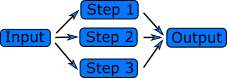The crucial thing that allows us to add the tires in parallel is that they are independent. Adding one tire does not prevent you from adding another, or require that any of the other tires are added. The workers operate on different parts of the car.

Data Dependency

Another example, and a common operation in scientific computing, is calculating the sum of a set of numbers. A simple implementation might look like this:

sum = 0
for number in numbers
   sum = sum + number

This is a very bad parallel algorithm! Every step, or iteration of the for loop, uses the same sum variable. To execute a step, the program needs to know the sum from the previous step.

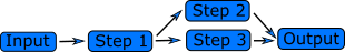
The important factor that determines whether steps can be run in parallel is data dependencies. In our sum example, every step depends on data from the previous step, the value of the sum variable. When attaching tires to a car, attaching one tire does not depend on attaching the others, so these steps can be done at the same time.

However, attaching the front tires both require that the axle is there. This step must be completed first, but the two tires can then be attached at the same time.

A part of the program that cannot be run in parallel is called a “serial region” and a part that can be run in parallel is called a “parallel region”. Any program will have some serial regions. In a good parallel program, most of the time is spent in parallel regions. The program can never run faster than the sum of the serial regions.

Serial and Parallel regions

Identify serial and parallel regions in the following algorithm

 vector_1[0] = 1;
 vector_1[1] = 1;
 for i in 2 ... 1000
   vector_1[i] = vector_1[i-1] + vector_1[i-2];

 for i in 0 ... 1000
   vector_2[i] = i;

 for i in 0 ... 1000
   vector_3[i] = vector_2[i] + vector_1[i];
   print("The sum of the vectors is.", vector_3[i]);

Solution

serial   | vector_0[0] = 1;
         | vector_1[1] = 1;
         | for i in 2 ... 1000
         |   vector_1[i] = vector_1[i-1] + vector_1[i-2];

parallel | for i in 0 ... 1000
         |   vector_2[i] = i;

parallel | for i in 0 ... 1000
         |   vector_3[i] = vector_2[i] + vector_1[i];
         |   print("The sum of the vectors is.", vector_3[i]);

The first and the second loop could also run at the same time.

In the first loop, every iteration depends on data from the previous two. In the second two loops, nothing in a step depends on any of the other steps.

Factors to consider for parallel algorithm

Amdahl’s Law

Using $N$ CPUs (or cores) doesn’t result in an $N$-times speedup. There is a theoretical limit in what parallelization can achieve, and it is encapsulated in “Amdahl’s Law”.

The time it takes to execute the program is roughly:

The $N_{\textrm{ranks}}$ here is the number of ranks, and $T_{\textrm{communications}}$ represents the time spent communicating between the ranks.

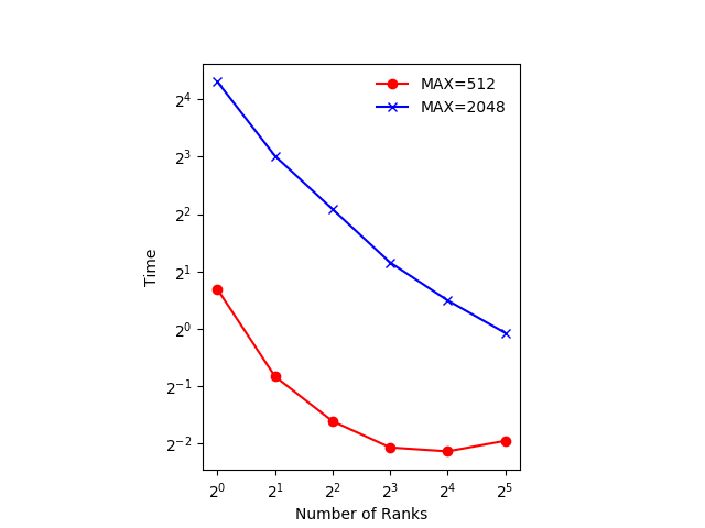
The other significant factors in the speed of a parallel program are communication speed, latency, and of course the number of parallel processes. In turn, the communication speed is determined by the amount of data one needs to send/receive, and the bandwidth of the underlying hardware for the communication. The latency consists of the software latency (how long the computer operating system needs in order to prepare for a communication), and the hardware latency (how long the hardware takes to send/receive even a small bit of data). For the same size problem, the time spent in communication is not significant when the number of ranks is small and the execution of parallel regions gets faster with the number of ranks. But if we keep increasing the number of ranks, the time spent in communication grows when multiple CPUs (or cores) are involved with communication (technically, this is called “global communication”).

L. Lamport’s Sequential Consistency

Message Passing based parallelization necessarily involves several “distributed” computing elements (CPUs or cores) which may operate on independent clocks. This can give wrong results, since the order of execution in an algorithm may not be the same as the corresponding serial execution performed by one CPU (or a core). This problem in parallelization is explained by L. Lamport in “How to make a Multiprocessor computer that correctly executes multiprocess programs”.

Consider a part of a program such as:

  y = 0;

  x = 1;

  y = 2;

  if(y < x) then stop;
  otherwise continue;

In a one CPU situation, there is no problem executing this part of the program and the program runs without stopping since the if statement is always false. Now, what if there are multiple CPUs (or cores) and the variables x and y are shared among these CPUs (or cores)? If the if statement happens before y = 2 in one of the CPUs (since x and y are shared, when one CPU updates y, the other CPU can’t touch it and just proceeds to the next step), the second CPU will stop running the program since it thinks y = 0 and x = 1 and the if statement is true for that CPU. So, sharing data among CPUs (or cores) in parallelization should be “sequentially consistent”.

Surface-to-Volume Ratio

In a parallel algorithm, the data which is handled by a CPU (or core) can be considered in two parts: the part the CPU needs that other CPUs (or cores) control, and a part that the CPU (or core) controls itself and can compute. The whole data which a CPU or a core computes is the sum of the two. The data under the control of the other CPUs (or cores) is called “surface” and the whole data is called “volume”.

The surface data requires communications. The more surface there is, the more communications among CPUs/cores is needed, and the longer the program will take to finish.

Due to Amdahl’s law, you want to minimize the number of communications for the same surface since each communication takes finite amount of time to prepare (latency). This suggests that the surface data be exchanged in one communication if possible, not small parts of the surface data exchanged in multiple communications. Of course, sequential consistency should be obeyed when the surface data is exchanged.

Key Points

• Algorithms can have parallelisable and non-parallelisable sections.

• A highly parallel algorithm may be slower on a single processor.

• The theoretical maximum speed is determined by the serial sections.

• The other main restriction is communication speed between the processes.